39 how to add percentage data labels in excel pie chart

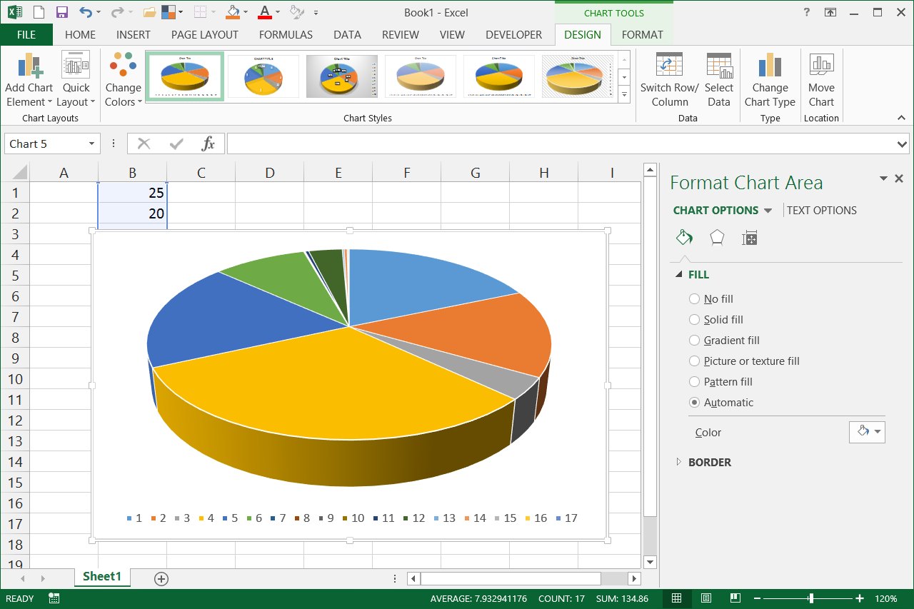
Pie Chart in Excel | How to Create Pie Chart - EDUCBA Step 1: Select the data to go to Insert, click on PIE, and select 3-D pie chart. Step 2: Now, it instantly creates the 3-D pie chart for you. Step 3: Right-click on the pie and select Add Data Labels. This will add all the values we are showing on the slices of the pie. How to Show Percentage in Pie Chart in Excel? - GeeksforGeeks Show percentage in a pie chart: The steps are as follows : Select the pie chart. Right-click on it. A pop-down menu will appear. Click on the Format Data Labels option. The Format Data Labels dialog box will appear. In this dialog box check the "Percentage" button and uncheck the Value button. This will replace the data labels in pie chart ...

How to show percentage in pie chart in Excel? - ExtendOffice Please do as follows to create a pie chart and show percentage in the pie slices. 1. Select the data you will create a pie chart based on, click Insert > I nsert Pie or Doughnut Chart > Pie. See screenshot: 2. Then a pie chart is created. Right click the pie chart and select Add Data Labels from the context menu. 3.

How to add percentage data labels in excel pie chart

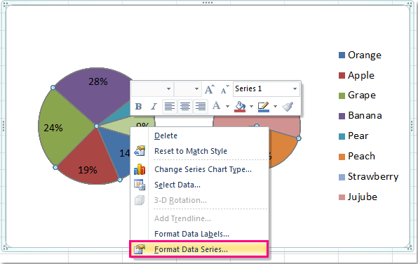
Inserting Data Label in the Color Legend of a pie chart Hi, I am trying to insert data labels (percentages) as part of the side colored legend, rather than on the pie chart itself, as displayed on the image ... There is no built-in way to do that, but you can use a trick: see Add Percent Values in Pie Chart Legend (Excel 2010) 0 Likes . Reply. Share. Share to LinkedIn; Share to Facebook; Share to ... How to Show Percentage in Excel Pie Chart (3 Ways) Display Percentage in Pie Chart by Using Format Data Labels. Another way of showing percentages in a pie chart is to use the Format Data Labels option. We can open the Format Data Labels window in the following two ways. 2.1 Using Chart Elements. To active the Format Data Labels window, follow the simple steps below. Steps: How To Make A Pie Chart With Percentages - PieProNation.com Right-click any slice within your Excel pie graph, and select Format Data Series from the context menu. On the Format Data Series pane, switch to the Series Options tab, and drag the Pie Explosion slider to increase or decrease gaps between the slices. Or, type the desired number directly in the percentage box:

How to add percentage data labels in excel pie chart. Microsoft Excel Tutorials: Add Data Labels to a Pie Chart To add the numbers from our E column (the viewing figures), left click on the pie chart itself to select it: The chart is selected when you can see all those blue circles surrounding it. Now right click the chart. You should get the following menu: From the menu, select Add Data Labels. New data labels will then appear on your chart: python - How to add value labels on a bar chart - Stack Overflow Firstly freq_series.plot returns an axis not a figure so to make my answer a little more clear I've changed your given code to refer to it as ax rather than fig to be more consistent with other code examples.. You can get the list of the bars produced in the plot from the ax.patches member. Then you can use the technique demonstrated in this matplotlib gallery example to add the labels using ... Excel 2010 pie chart data labels in case of "Best Fit" Based on my tested in Excel 2010, the data labels in the "Inside" or "Outside" is based on the data source. If the gap between the data is big, the data labels and leader lines is "outside" the chart. And if the gap between the data is small, the data labels and leader lines is "inside" the chart. Regards, George Zhao. TechNet Community Support. Show values & percentages in a pie chart? - MrExcel Message Board 2. Sep 17, 2014. #3. cyrilbrd said: What version of excel are you using? Add labels, select labels, select format data labels, go to labels options, tick both Value and Percentage, use the separator of your liking. Would that work for you? Click to expand... How about if I want to show both the value but the percentage is in bracket for example ...

Change the format of data labels in a chart Tip: To switch from custom text back to the pre-built data labels, click Reset Label Text under Label Options. To format data labels, select your chart, and then in the Chart Design tab, click Add Chart Element > Data Labels > More Data Label Options. Click Label Options and under Label Contains, pick the options you want. How to Create and Format a Pie Chart in Excel - Lifewire To create a pie chart, highlight the data in cells A3 to B6 and follow these directions: On the ribbon, go to the Insert tab. Select Insert Pie Chart to display the available pie chart types. Hover over a chart type to read a description of the chart and to preview the pie chart. Choose a chart type. Pie of Pie Chart in Excel - Inserting, Customizing, Formatting Inserting a Pie of Pie Chart. Let us say we have the sales of different items of a bakery. Below is the data:-. To insert a Pie of Pie chart:-. Select the data range A1:B7. Enter in the Insert Tab. Select the Pie button, in the charts group. Select Pie of Pie chart in the 2D chart section. How to display percentage labels in pie chart in Excel - YouTube to display percentage labels in pie chart in Excel

Display percentage values on pie chart in a paginated report ... To display percentage values as labels on a pie chart. Add a pie chart to your report. For more information, see Add a Chart to a Report (Report Builder and SSRS). On the design surface, right-click on the pie and select Show Data Labels. The data labels should appear within each slice on the pie chart. On the design surface, right-click on the ... How to show data label in "percentage" instead of - Microsoft Community Select Format Data Labels. Select Number in the left column. Select Percentage in the popup options. In the Format code field set the number of decimal places required and click Add. (Or if the table data in in percentage format then you can select Link to source.) Click OK. Regards, OssieMac. Report abuse. How to Add Percentages to Excel Bar Chart If we would like to add percentages to our bar chart, we would need to have percentages in the table in the first place. We will create a column right to the column points in which we would divide the points of each player with the total points of all players. We will select range A1:C8 and go to Insert >> Charts >> 2-D Column >> Stacked Column: Creating Pie Chart and Adding/Formatting Data Labels (Excel) Creating Pie Chart and Adding/Formatting Data Labels (Excel) Creating Pie Chart and Adding/Formatting Data Labels (Excel)

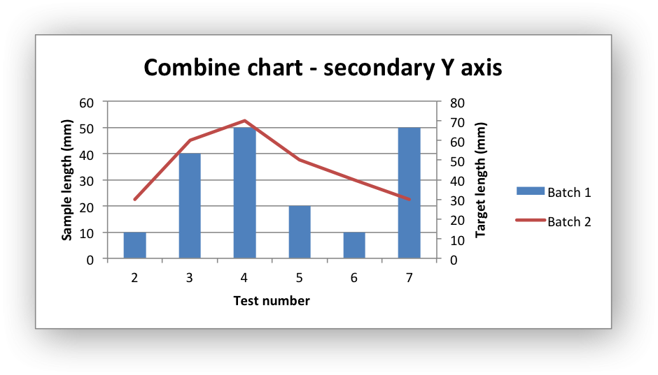
How to create a chart with both percentage and value in Excel? Create a chart with both percentage and value in Excel. To solve this task in Excel, please do with the following step by step: 1. Select the data range that you want to create a chart but exclude the percentage column, and then click Insert > Insert Column or Bar Chart > 2-D Clustered Column Chart, see screenshot: 2.

Add or remove data labels in a chart - support.microsoft.com On the Design tab, in the Chart Layouts group, click Add Chart Element, choose Data Labels, and then click None. Click a data label one time to select all data labels in a data series or two times to select just one data label that you want to delete, and then press DELETE. Right-click a data label, and then click Delete.

How to Make a Pie Chart in Excel & Add Rich Data Labels to The Chart! Creating and formatting the Pie Chart. 1) Select the data. 2) Go to Insert> Charts> click on the drop-down arrow next to Pie Chart and under 2-D Pie, select the Pie Chart, shown below. 3) Chang the chart title to Breakdown of Errors Made During the Match, by clicking on it and typing the new title.

Pie Chart - Show Percentage - Excel & Google Sheets Change to Percentage. This will show the "Values" of the data labels. The next step is changing these to percentages instead. Right click on the new labels. Select Format Data Labels. 3. Uncheck box next to Value. 4. Check box next to Percentage.

How to Add Percentage Axis to Chart in Excel To do this, we will select the whole table again, and then go to Insert >> Charts >> 2-D Columns: To show percentages on a second axis, we first need to click anywhere on the orange bars that we have on our graph (this is not easy in this example as they are rather small). Once we do, we will right-click on it, and then select Format Data Series:

adding decimal places to percentages in pie charts I am V. Arya, Independent Advisor, to work with you on this issue. Right click on your % label - Format Data labels. Beneath Number choose percentage as category. Report abuse. 39 people found this reply helpful. ·.

Add Percent Values in Pie Chart Legend (Excel 2010) In Row 4 enter the formula = A1 & " " & Text (A3,"0%") Copy this across. No in your Pie chart. Locate Select Data on the Design Tab. Click the Edit button under Horizontal (Category) Axis Labels and set it to the A4 to C4 cells you've just created. Hope this helps.

Share :